Underwater Networks Handbook

The hello world of the networking world is the ALOHA MAC protocol. The protocol is very simple: transmit a frame as soon as data arrives, without worrying about whether any other node is transmitting. While this behavior is straightforward to describe, simulating it accurately requires some thought.

Let’s say we want to simulate a network with ALOHA MAC. On each node, we expect data to arrive randomly, with a known average arrival rate. The total number of data "chunks" arriving per unit time across the network is termed as offered load . As soon as a data chunk arrives, the node transmits it to a randomly chosen destination node (other than itself). The number of successfully delivered data chunks per unit time, across the entire network, is called the throughput . We are interested to study how the throughput varies as a function of offered load.

ALOHA has been extensively studied in literature, and its theoretical performance is well known. In order to simulate a network that can be compared against theory, we need to ensure that our simulation matches the assumptions made in the theoretical derivations:

Assumptions 2 and 4 together form a model called the protocol channel model. We tell the simulator to adopt this model:

Underwater acoustic modems are usually half-duplex, and the default modem model in the simulator is the HalfDuplexModem , so we shouldn’t need to do anything special for assumption 3. However, the HalfDuplexModem is smart enough to delay a transmission if another frame is being transmitted or received by the node, to avoid losing the other frame. While this is usually a good thing to do, it will violate assumption 3 and give us results that don’t agree with theory. To match the theoretical behavior, we have to stop any ongoing transmission or reception, when new data arrives for transmission:

The offered load and throughput are usually normalized by the number of frames that can be supported by the channel per unit time. By setting the frame duration to be one second, we ensure that the normalization factor is 1 (one packet can be transitted per second without collision). To do this, we set up the simulated modem to have no header/preamble overheads, and exactly 1 second worth of data that it can carry in a frame:

A Poisson process (assumption 1) is easily simulated using the PoissonBehavior available in fjåge. Assumption 5 can also be easily met by placing all nodes at the same location.

Now let’s put a first version of our script together to simulate a 4-node ALOHA network:

The script is easy to understand. In a 2-hour long simulation, we iterate over the list of nodes, and create each node at the origin. Each node adds a PoissonBehavior to generate random traffic at a rate corresponding to the offered load setting. The parameter of the Poisson behavior is the average time between events in milliseconds, which we compute based on the arrival rate. The destination for each transmission is randomly chosen from the list of nodes excluding the transmitting node. Once the simulation is completed, statistics are printed. The trace object is automatically defined by the simulator to collect typically required statistics.

Open Unet IDE ( bin/unet sim ), create a new simulation script in the scripts folder, copy this code in, and run it. Within a few seconds, you should see the results:

Since this is a Monte-Carlo simulation driven by a random number generator, the statistics you see will be similar, but not identical. A total of 1459 frames were transmitted, and 984 of them were successfully received. The measured offered load was 0.2026, and the throughput was 0.1367.

Hang on a minute! The simulation was meant to run for 2 hours, but it finished in less than 3 seconds!!

That’s because we ran the simulation in a discrete event simulation mode (it is the default mode, if we don’t set platform = RealTimePlatform ). We could have explicitly set it ( platform = DiscreteEventSimulator ), if we wanted. Now that we can run hours worth of simulations in seconds, we can go ahead and measure ALOHA throughput at various load settings:

Other than the pretty printing to tabulate the output, you’ll see that we have added a trace.warmup time. This is to ensure that we only collect statistics after the simulation has reached steady state (in this case, after 15 minutes of simulation time).

A slightly beautified copy of the above code is available in the samples/aloha.groovy script. You can either run that, or run the above code. You should see something like this output:

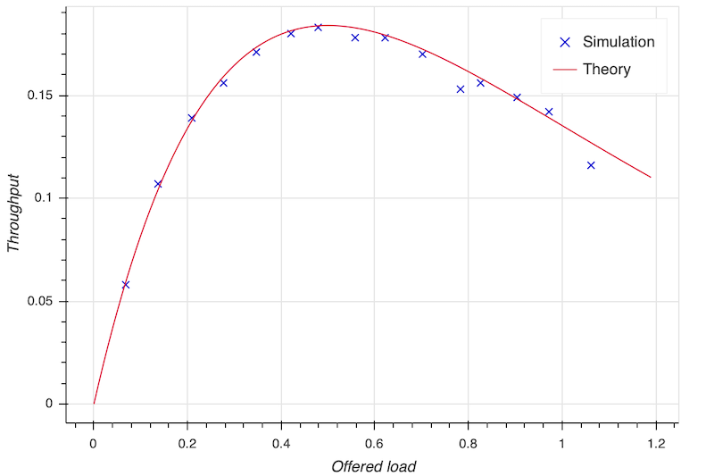
As expected from the ALOHA protocol, the maximum throughput of about 0.18 is reached at an offered load of about 0.5. We plot this against the theoretical ALOHA performance curve ( y = x exp(-2x) ) in Figure 16 .

When a simulation is run, usually two files are produced.

Since UnetStack 3.3.0, the default trace file is stored in a rich JSON format.

When running a simulation, a JSON trace file logs/trace.json is automatically generated. This file contains a detailed trace for every event in the network stack, on each node. You can even enable trace file generation on real modems and other Unet nodes (using EventTracer.enable() ), and later combine the traces from multiple nodes to analyze network protocol operation and performance.

A small extract from a typical trace file is shown below:

The trace is organized into a hierarchy of groups, each describing a simulation run or the execution of specific commands. A group consists of a sequence of events, with each event providing information on time of event, component (agent running on a node), thread ID, stimulus and response. The stimulus is typically a message received from another agent, and response a message sent to another agent. The thread ID ties multiple events, potentially across multiple agents and nodes, but with the same root cause together.

An experimental automated trace analysis tool can be used to produce sequence diagrams from JSON trace files.

Integrating the event tracing framework into your own agents is simple. All you need to do is to wrap messages that you generate in response to a stimulus with a trace() call. Some examples:

The legacy trace file format is similar to the NS2 NAM trace. Since UnetStack 3.3.0, this format is no longer the default, but can be enabled easily in your simulation script if you need it:

The trace file contains information about all packet creation, transmission, reception and drop events. It also contains details of node motion. The tracer also computes basic statistics including queued packet count, transmitted packet count, received packet count, dropped packet count, offered load, actual load, average packet latency and normalized throughput. An extract from the trace file is shown below:

Lines starting with n log node locations/motion. Lines starting with + denote packet arrival into the transmit queue. Lines starting with - log packet removal from the transmit queue, i.e., transmission. Lines starting with r denote packet reception (or overhearing). Lines starting with d log packet drops, and specify a reason for the drop. CLEAR indicates a packet transmission/reception abort due to a ClearReq request. COLLISION indicates that the packet was dropped because the node was busy receiving or transmitting another packet. BAD_FRAME indicates that the packet was corrupted (possibly due to interference from a colliding packet).

For more details on the trace file format, see NS2 NAM trace format .